@eagleoutice/flowr - v2.13.2

![]()
![]()

![]()
flowR is a sophisticated, static dataflow analyzer for the R programming language, available for VSCode, Positron, RStudio, and Docker. It offers a wide variety of features, for example:
-
🐞 code linting
Analyze your R scripts for common issues and potential bugs (see the wiki page for more information on the currently supported linters).Example: Linting code with flowR
To lint your code, you can use the REPL or the Visual Studio Code extension (see vscode-flowr#283).
$ docker run -it --rm eagleoutice/flowr # or npm run flowr
flowR repl v2.13.0, R grammar v14 (tree-sitter engine)
R> :query @linter "read.csv(\"/root/x.txt\")"Output
Query: linter (9 ms) ╰ Deprecated Functions (deprecated-functions): no findings ╰ File Path Validity (file-path-validity): ╰ certain: ╰ Path `/root/x.txt` at 1.1-23 ╰ Metadata: totalReads: 1, totalUnknown: 0, totalWritesBeforeAlways: 0, totalValid: 0, searchTimeMs: 1, processTimeMs: 0 ╰ Seeded Randomness (seeded-randomness): no findings ╰ Absolute Paths (absolute-file-paths): ╰ certain: ╰ Path `/root/x.txt` at 1.1-23 ╰ Metadata: totalConsidered: 1, totalUnknown: 0, searchTimeMs: 1, processTimeMs: 0 ╰ Unused Definitions (unused-definitions): no findings ╰ Network Functions (network-functions): no findings ╰ Dataframe Access Validation (dataframe-access-validation): no findings ╰ Dead Code (dead-code): no findings ╰ Useless Loops (useless-loop): no findings ╰ Problematic inputs (problematic-inputs): no findings ╰ Stop without call.=False argument (stop-call): no findings ╰ Roxygen Arguments (roxygen-arguments): no findings ╰ No Leaked Credentials (no-leaked-credentials): no findings ╰ Undefined Symbol (undefined-symbol): no findings All queries together required ≈9 ms (1ms accuracy, total 9 ms)The linter will analyze the code and return any issues found. Formatted more nicely, this returns:
[ { "type": "linter" } ](This can be shortened to
@linterwhen used with the REPL command:query).Results (prettified and summarized):
Query: linter (11 ms)
╰ Deprecated Functions (deprecated-functions): no findings
╰ File Path Validity (file-path-validity):
╰ certain:
╰ Path/root/x.txtat 1.1-23
╰ Metadata: totalReads: 1, totalUnknown: 0, totalWritesBeforeAlways: 0, totalValid: 0, searchTimeMs: 1, processTimeMs: 0
╰ Seeded Randomness (seeded-randomness): no findings
╰ Absolute Paths (absolute-file-paths):
╰ certain:
╰ Path/root/x.txtat 1.1-23
╰ Metadata: totalConsidered: 1, totalUnknown: 0, searchTimeMs: 0, processTimeMs: 0
╰ Unused Definitions (unused-definitions): no findings
╰ Network Functions (network-functions): no findings
╰ Dataframe Access Validation (dataframe-access-validation): no findings
╰ Dead Code (dead-code): no findings
╰ Useless Loops (useless-loop): no findings
╰ Problematic inputs (problematic-inputs): no findings
╰ Stop without call.=False argument (stop-call): no findings
╰ Roxygen Arguments (roxygen-arguments): no findings
╰ No Leaked Credentials (no-leaked-credentials): no findings
╰ Undefined Symbol (undefined-symbol): no findings
All queries together required ≈11 ms (1ms accuracy, total 12 ms)Show Detailed Results as Json
The analysis required 12.4 ms (including parsing and normalization and the query) within the generation environment.
In general, the JSON contains the Ids of the nodes in question as they are present in the normalized AST or the dataflow graph of flowR. Please consult the Interface wiki page for more information on how to get those.
{
"linter": {
"results": {
"deprecated-functions": {
"results": [],
".meta": {
"totalCalls": 0,
"totalFunctionDefinitions": 0,
"searchTimeMs": 3,
"processTimeMs": 1
}
},
"file-path-validity": {
"results": [
{
"involvedId": 3,
"loc": [
1,
1,
1,
23
],
"filePath": "/root/x.txt",
"certainty": "certain"
}
],
".meta": {
"totalReads": 1,
"totalUnknown": 0,
"totalWritesBeforeAlways": 0,
"totalValid": 0,
"searchTimeMs": 1,
"processTimeMs": 0
}
},
"seeded-randomness": {
"results": [],
".meta": {
"consumerCalls": 0,
"callsWithFunctionProducers": 0,
"callsWithAssignmentProducers": 0,
"callsWithNonConstantProducers": 0,
"callsWithOtherBranchProducers": 0,
"searchTimeMs": 1,
"processTimeMs": 0
}
},
"absolute-file-paths": {
"results": [
{
"certainty": "certain",
"filePath": "/root/x.txt",
"loc": [
1,
1,
1,
23
]
}
],
".meta": {
"totalConsidered": 1,
"totalUnknown": 0,
"searchTimeMs": 0,
"processTimeMs": 0
}
},
"unused-definitions": {
"results": [],
".meta": {
"totalConsidered": 0,
"searchTimeMs": 0,
"processTimeMs": 1
}
},
"network-functions": {
"results": [],
".meta": {
"totalCalls": 0,
"totalFunctionDefinitions": 0,
"searchTimeMs": 0,
"processTimeMs": 0
}
},
"dataframe-access-validation": {
"results": [],
".meta": {
"numOperations": 0,
"numAccesses": 0,
"totalAccessed": 0,
"searchTimeMs": 0,
"processTimeMs": 1
}
},
"dead-code": {
"results": [],
".meta": {
"searchTimeMs": 0,
"processTimeMs": 0
}
},
"useless-loop": {
"results": [],
".meta": {
"numOfUselessLoops": 0,
"searchTimeMs": 0,
"processTimeMs": 0
}
},
"problematic-inputs": {
"results": [],
".meta": {
"searchTimeMs": 0,
"processTimeMs": 0
}
},
"stop-call": {
"results": [],
".meta": {
"consideredNodes": 0,
"searchTimeMs": 0,
"processTimeMs": 0
}
},
"roxygen-arguments": {
"results": [],
".meta": {
"searchTimeMs": 0,
"processTimeMs": 0
}
},
"no-leaked-credentials": {
"results": [],
".meta": {
"totalChecked": 0,
"searchTimeMs": 0,
"processTimeMs": 0
}
},
"undefined-symbol": {
"results": [],
".meta": {
"totalFunctionCalls": 1,
"totalVariableUses": 0,
"suppressed": {
"installed": 0,
"loadedPackage": 0,
"enclosingScope": 0,
"nonStandardEval": 0,
"subscript": 0
},
"searchTimeMs": 0,
"processTimeMs": 3
}
}
},
".meta": {
"timing": 11
}
},
".meta": {
"timing": 11
}
} -
🍕 program slicing
Given a point of interest like the visualization of a plot, flowR reduces the program to just the parts which are relevant for the computation of the point of interest.Example: Slicing with flowR
The simplest way to retrieve slices is with flowR's Visual Studio Code extension. However, you can slice using the REPL as well. This can help you if you want to reuse specific parts of an existing analysis within another context or if you want to understand what is happening in the code.
For this, let's have a look at the example file, located at test/testfiles/example.R:
sum <- 0
product <- 1
w <- 7
N <- 10
for (i in 1:(N-1)) {
sum <- sum + i + w
product <- product * i
}
cat("Sum:", sum, "\n")
cat("Product:", product, "\n")Let's suppose we are interested only in the
sumwhich is printed in line 11. To get a slice for this, you can use the following command:$ docker run -it --rm eagleoutice/flowr # or npm run flowr
flowR repl v2.13.0, R grammar v14 (tree-sitter engine)
R> :query @static-slice (11@sum) file://test/testfiles/example.ROutput
sum <- 0 w <- 7 N <- 10 for(i in 1:(N-1)) sum <- sum + i + w sum All queries together required ≈6 ms (1ms accuracy, total 7 ms) -
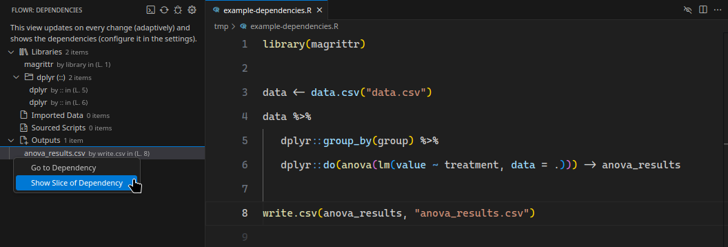
📚 dependency analysis
Given your analysis project, flowR offers a plethora of so-called queries to get more information about your code. An important query is the dependencies query, which shows you the library your project needs, the data files it reads, the scripts it sources, and the data it outputs.Example: Dependency Analysis with flowR
The following showcases the dependency view of the Visual Studio Code extension:
-
🚀 fast call-graph, data-, and control-flow graphs
Within just 104.8 ms (as of Jul 20, 2026), flowR can analyze the data- and control-flow of the average real-world R script. See the benchmarks for more information, and consult the wiki pages for more details on the dataflow graphs as well as call graphs.Example: Generating a dataflow graph with flowR
You can investigate flowR's analyses using the REPL. Commands like
:dataflow*allow you to view a dataflow graph for a given R script.Let's have a look at the following example:
sum <- 0
product <- 1
w <- 7
N <- 10
for (i in 1:(N-1)) {
sum <- sum + i + w
product <- product * i
}
cat("Sum:", sum, "\n")
cat("Product:", product, "\n")To get the dataflow graph for this script, you can use the following command:
$ docker run -it --rm eagleoutice/flowr # or npm run flowr
flowR repl v2.13.0, R grammar v14 (tree-sitter engine)
R> :dataflow* test/testfiles/example.ROutput
'test/testfiles/example.R' looks like a path, analyzing file://test/testfiles/example.R (repl.autoUseFileProtocol is set). https://mermaid.live/view#base64:eyJjb2RlIjoiZmxvd2NoYXJ0IEJUXG4gICAgMXt7XCJgKiM5MTtSTnVtYmVyIzkzOyogKiowKipcbiAgICAgICoxLjgqICgqKmlkOiAxKiopYFwifX1cbiAgICUlIE5vIGVkZ2VzIGZvdW5kIGZvciAxXG4gICAgMFtcImAqIzkxO1JTeW1ib2wjOTM7KiAqKnN1bSoqXG4gICAgICAqMS4xLTMqICgqKmlkOiAwKiosIHY6IDEpYFwiXVxuICAgIDJbW1wiYCojOTE7UkJpbmFyeU9wIzkzOyogYmFzZSM1ODsjNTg7KiojNjA7IzQ1OyoqXG4gICAgICAqMS4xLTgqICgqKmlkOiAyKiopXG4gICAgYXJnOiAoMCwgMSlgXCJdXVxuICAgIGJ1aWx0LWluOl8tW1wiYEJ1aWx0LUluOlxuIzYwOyM0NTtgXCJdXG4gICAgc3R5bGUgYnVpbHQtaW46Xy0gc3Ryb2tlOmdyYXksZmlsbDpncmF5LHN0cm9rZS13aWR0aDoycHgsb3BhY2l0eTouODtcbiAgICA0e3tcImAqIzkxO1JOdW1iZXIjOTM7KiAqKjEqKlxuICAgICAgKjIuMTIqICgqKmlkOiA0KiopYFwifX1cbiAgICUlIE5vIGVkZ2VzIGZvdW5kIGZvciA0XG4gICAgM1tcImAqIzkxO1JTeW1ib2wjOTM7KiAqKnByb2R1Y3QqKlxuICAgICAgKjIuMS03KiAoKippZDogMyoqLCB2OiA0KWBcIl1cbiAgICA1W1tcImAqIzkxO1JCaW5hcnlPcCM5MzsqIGJhc2UjNTg7IzU4OyoqIzYwOyM0NTsqKlxuICAgICAgKjIuMS0xMiogKCoqaWQ6IDUqKilcbiAgICBhcmc6ICgzLCA0KWBcIl1dXG4gICAgN3t7XCJgKiM5MTtSTnVtYmVyIzkzOyogKio3KipcbiAgICAgICozLjYqICgqKmlkOiA3KiopYFwifX1cbiAgICUlIE5vIGVkZ2VzIGZvdW5kIGZvciA3XG4gICAgNltcImAqIzkxO1JTeW1ib2wjOTM7KiAqKncqKlxuICAgICAgKjMuMSogKCoqaWQ6IDYqKiwgdjogNylgXCJdXG4gICAgOFtbXCJgKiM5MTtSQmluYXJ5T3AjOTM7KiBiYXNlIzU4OyM1ODsqKiM2MDsjNDU7KipcbiAgICAgICozLjEtNiogKCoqaWQ6IDgqKilcbiAgICBhcmc6ICg2LCA3KWBcIl1dXG4gICAgMTB7e1wiYCojOTE7Uk51bWJlciM5MzsqICoqMTAqKlxuICAgICAgKjQuNi03KiAoKippZDogMTAqKilgXCJ9fVxuICAgJSUgTm8gZWRnZXMgZm91bmQgZm9yIDEwXG4gICAgOVtcImAqIzkxO1JTeW1ib2wjOTM7KiAqKk4qKlxuICAgICAgKjQuMSogKCoqaWQ6IDkqKiwgdjogMTApYFwiXVxuICAgIDExW1tcImAqIzkxO1JCaW5hcnlPcCM5MzsqIGJhc2UjNTg7IzU4OyoqIzYwOyM0NTsqKlxuICAgICAgKjQuMS03KiAoKippZDogMTEqKilcbiAgICBhcmc6ICg5LCAxMClgXCJdXVxuICAgIDEyW1wiYCojOTE7UlN5bWJvbCM5MzsqICoqaSoqXG4gICAgICAqNi42KiAoKippZDogMTIqKiwgdjogMjApYFwiXVxuICAgIDEze3tcImAqIzkxO1JOdW1iZXIjOTM7KiAqKjEqKlxuICAgICAgKjYuMTEqICgqKmlkOiAxMyoqKWBcIn19XG4gICAlJSBObyBlZGdlcyBmb3VuZCBmb3IgMTNcbiAgICAxNihbXCJgKiM5MTtSU3ltYm9sIzkzOyogKipOKipcbiAgICAgICo2LjE0KiAoKippZDogMTYqKilgXCJdKVxuICAgIDE3e3tcImAqIzkxO1JOdW1iZXIjOTM7KiAqKjEqKlxuICAgICAgKjYuMTYqICgqKmlkOiAxNyoqKWBcIn19XG4gICAlJSBObyBlZGdlcyBmb3VuZCBmb3IgMTdcbiAgICAxOFtbXCJgKiM5MTtSQmluYXJ5T3AjOTM7KiBiYXNlIzU4OyM1ODsqKiM0NTsqKlxuICAgICAgKjYuMTQtMTYqICgqKmlkOiAxOCoqKVxuICAgIGFyZzogKDE2LCAxNylgXCJdXVxuICAgIGJ1aWx0LWluOi1bXCJgQnVpbHQtSW46XG4jNDU7YFwiXVxuICAgIHN0eWxlIGJ1aWx0LWluOi0gc3Ryb2tlOmdyYXksZmlsbDpncmF5LHN0cm9rZS13aWR0aDoycHgsb3BhY2l0eTouODtcbiAgICAxOVtbXCJgKiM5MTtSRXhwcmVzc2lvbkxpc3QjOTM7KiBiYXNlIzU4OyM1ODsqKigqKlxuICAgICAgKjYuMTMqICgqKmlkOiAxOSoqKVxuICAgIGFyZzogKDE4KWBcIl1dXG4gICAgMjBbW1wiYCojOTE7UkJpbmFyeU9wIzkzOyogYmFzZSM1ODsjNTg7KiojNTg7KipcbiAgICAgICo2LjExLTE3KiAoKippZDogMjAqKilcbiAgICBhcmc6ICgxMywgMTkpYFwiXV1cbiAgICBidWlsdC1pbjo6W1wiYEJ1aWx0LUluOlxuIzU4O2BcIl1cbiAgICBzdHlsZSBidWlsdC1pbjo6IHN0cm9rZTpncmF5LGZpbGw6Z3JheSxzdHJva2Utd2lkdGg6MnB4LG9wYWNpdHk6Ljg7XG4gICAgMjQoW1wiYCojOTE7UlN5bWJvbCM5MzsqICoqc3VtKipcbiAgICAgICo3LjEwLTEyKiAoKippZDogMjQqKiwgMzYrKWBcIl0pXG4gICAgMjUoW1wiYCojOTE7UlN5bWJvbCM5MzsqICoqaSoqXG4gICAgICAqNy4xNiogKCoqaWQ6IDI1KiosIDM2KylgXCJdKVxuICAgIDI2W1tcImAqIzkxO1JCaW5hcnlPcCM5MzsqIGJhc2UjNTg7IzU4OyoqIzQzOyoqXG4gICAgICAqNy4xMC0xNiogKCoqaWQ6IDI2KiosIDM2KylcbiAgICBhcmc6ICgyNCwgMjUpYFwiXV1cbiAgICBidWlsdC1pbjpfW1wiYEJ1aWx0LUluOlxuIzQzO2BcIl1cbiAgICBzdHlsZSBidWlsdC1pbjpfIHN0cm9rZTpncmF5LGZpbGw6Z3JheSxzdHJva2Utd2lkdGg6MnB4LG9wYWNpdHk6Ljg7XG4gICAgMjcoW1wiYCojOTE7UlN5bWJvbCM5MzsqICoqdyoqXG4gICAgICAqNy4yMCogKCoqaWQ6IDI3KiosIDM2KylgXCJdKVxuICAgIDI4W1tcImAqIzkxO1JCaW5hcnlPcCM5MzsqIGJhc2UjNTg7IzU4OyoqIzQzOyoqXG4gICAgICAqNy4xMC0yMCogKCoqaWQ6IDI4KiosIDM2KylcbiAgICBhcmc6ICgyNiwgMjcpYFwiXV1cbiAgICAyM1tcImAqIzkxO1JTeW1ib2wjOTM7KiAqKnN1bSoqXG4gICAgICAqNy4zLTUqICgqKmlkOiAyMyoqLCAzNissIHY6IDI4KWBcIl1cbiAgICAyOVtbXCJgKiM5MTtSQmluYXJ5T3AjOTM7KiBiYXNlIzU4OyM1ODsqKiM2MDsjNDU7KipcbiAgICAgICo3LjMtMjAqICgqKmlkOiAyOSoqLCAzNispXG4gICAgYXJnOiAoMjMsIDI4KWBcIl1dXG4gICAgMzEoW1wiYCojOTE7UlN5bWJvbCM5MzsqICoqcHJvZHVjdCoqXG4gICAgICAqOC4xNC0yMCogKCoqaWQ6IDMxKiosIDM2KylgXCJdKVxuICAgIDMyKFtcImAqIzkxO1JTeW1ib2wjOTM7KiAqKmkqKlxuICAgICAgKjguMjQqICgqKmlkOiAzMioqLCAzNispYFwiXSlcbiAgICAzM1tbXCJgKiM5MTtSQmluYXJ5T3AjOTM7KiBiYXNlIzU4OyM1ODsqKiM0MjsqKlxuICAgICAgKjguMTQtMjQqICgqKmlkOiAzMyoqLCAzNispXG4gICAgYXJnOiAoMzEsIDMyKWBcIl1dXG4gICAgMzBbXCJgKiM5MTtSU3ltYm9sIzkzOyogKipwcm9kdWN0KipcbiAgICAgICo4LjMtOSogKCoqaWQ6IDMwKiosIDM2KywgdjogMzMpYFwiXVxuICAgIDM0W1tcImAqIzkxO1JCaW5hcnlPcCM5MzsqIGJhc2UjNTg7IzU4OyoqIzYwOyM0NTsqKlxuICAgICAgKjguMy0yNCogKCoqaWQ6IDM0KiosIDM2KylcbiAgICBhcmc6ICgzMCwgMzMpYFwiXV1cbiAgICAzNVtbXCJgKiM5MTtSRXhwcmVzc2lvbkxpc3QjOTM7KiBiYXNlIzU4OyM1ODsqKiMxMjM7KipcbiAgICAgICo2LjIwKiAoKippZDogMzUqKiwgMzYrKVxuICAgIGFyZzogKDI5LCAzNClgXCJdXVxuICAgIDM2W1tcImAqIzkxO1JGb3JMb29wIzkzOyogYmFzZSM1ODsjNTg7Kipmb3IqKlxuICAgICAgKjYuMS05LjEqICgqKmlkOiAzNioqKVxuICAgIGFyZzogKDEyLCAyMCwgMzUpYFwiXV1cbiAgICBidWlsdC1pbjpmb3JbXCJgQnVpbHQtSW46XG5mb3JgXCJdXG4gICAgc3R5bGUgYnVpbHQtaW46Zm9yIHN0cm9rZTpncmF5LGZpbGw6Z3JheSxzdHJva2Utd2lkdGg6MnB4LG9wYWNpdHk6Ljg7XG4gICAgMzh7e1wiYCojOTE7UlN0cmluZyM5MzsqICoqIzM0O1N1bSM1ODsjMzQ7KipcbiAgICAgICoxMS41LTEwKiAoKippZDogMzgqKilgXCJ9fVxuICAgJSUgTm8gZWRnZXMgZm91bmQgZm9yIDM4XG4gICAgNDAoW1wiYCojOTE7UlN5bWJvbCM5MzsqICoqc3VtKipcbiAgICAgICoxMS4xMy0xNSogKCoqaWQ6IDQwKiopYFwiXSlcbiAgICBidWlsdC1pbjpzdW1bXCJgQnVpbHQtSW46XG5zdW1gXCJdXG4gICAgc3R5bGUgYnVpbHQtaW46c3VtIHN0cm9rZTpncmF5LGZpbGw6Z3JheSxzdHJva2Utd2lkdGg6MnB4LG9wYWNpdHk6Ljg7XG4gICAgNDJ7e1wiYCojOTE7UlN0cmluZyM5MzsqICoqIzM0O1xuIzM0OyoqXG4gICAgICAqMTEuMTgtMjEqICgqKmlkOiA0MioqKWBcIn19XG4gICAlJSBObyBlZGdlcyBmb3VuZCBmb3IgNDJcbiAgICA0NFtbXCJgKiM5MTtSRnVuY3Rpb25DYWxsIzkzOyogYmFzZSM1ODsjNTg7KipjYXQqKlxuICAgICAgKjExLjEtMjIqICgqKmlkOiA0NCoqKVxuICAgIGFyZzogKDM4LCA0MCwgNDIpYFwiXV1cbiAgICBidWlsdC1pbjpjYXRbXCJgQnVpbHQtSW46XG5jYXRgXCJdXG4gICAgc3R5bGUgYnVpbHQtaW46Y2F0IHN0cm9rZTpncmF5LGZpbGw6Z3JheSxzdHJva2Utd2lkdGg6MnB4LG9wYWNpdHk6Ljg7XG4gICAgNDZ7e1wiYCojOTE7UlN0cmluZyM5MzsqICoqIzM0O1Byb2R1Y3QjNTg7IzM0OyoqXG4gICAgICAqMTIuNS0xNCogKCoqaWQ6IDQ2KiopYFwifX1cbiAgICUlIE5vIGVkZ2VzIGZvdW5kIGZvciA0NlxuICAgIDQ4KFtcImAqIzkxO1JTeW1ib2wjOTM7KiAqKnByb2R1Y3QqKlxuICAgICAgKjEyLjE3LTIzKiAoKippZDogNDgqKilgXCJdKVxuICAgIDUwe3tcImAqIzkxO1JTdHJpbmcjOTM7KiAqKiMzNDtcbiMzNDsqKlxuICAgICAgKjEyLjI2LTI5KiAoKippZDogNTAqKilgXCJ9fVxuICAgJSUgTm8gZWRnZXMgZm91bmQgZm9yIDUwXG4gICAgNTJbW1wiYCojOTE7UkZ1bmN0aW9uQ2FsbCM5MzsqIGJhc2UjNTg7IzU4OyoqY2F0KipcbiAgICAgICoxMi4xLTMwKiAoKippZDogNTIqKilcbiAgICBhcmc6ICg0NiwgNDgsIDUwKWBcIl1dXG4gICAgMCAtLT58XCJkZWZpbmVkLWJ5XCJ8IDFcbiAgICAwIC0tPnxcImRlZmluZWQtYnlcInwgMlxuICAgIDIgLS0+fFwicmVhZHMsIGFyZ1wifCAxXG4gICAgMiAtLT58XCJyZXR1cm5zLCBhcmdcInwgMFxuICAgIDIgLS4tPnxcInJlYWRzLCBjYWxsc1wifCBidWlsdC1pbjpfLVxuICAgIGxpbmtTdHlsZSA0IHN0cm9rZTpncmF5O1xuICAgIDMgLS0+fFwiZGVmaW5lZC1ieVwifCA0XG4gICAgMyAtLT58XCJkZWZpbmVkLWJ5XCJ8IDVcbiAgICA1IC0tPnxcInJlYWRzLCBhcmdcInwgNFxuICAgIDUgLS0+fFwicmV0dXJucywgYXJnXCJ8IDNcbiAgICA1IC0uLT58XCJyZWFkcywgY2FsbHNcInwgYnVpbHQtaW46Xy1cbiAgICBsaW5rU3R5bGUgOSBzdHJva2U6Z3JheTtcbiAgICA2IC0tPnxcImRlZmluZWQtYnlcInwgN1xuICAgIDYgLS0+fFwiZGVmaW5lZC1ieVwifCA4XG4gICAgOCAtLT58XCJyZWFkcywgYXJnXCJ8IDdcbiAgICA4IC0tPnxcInJldHVybnMsIGFyZ1wifCA2XG4gICAgOCAtLi0+fFwicmVhZHMsIGNhbGxzXCJ8IGJ1aWx0LWluOl8tXG4gICAgbGlua1N0eWxlIDE0IHN0cm9rZTpncmF5O1xuICAgIDkgLS0+fFwiZGVmaW5lZC1ieVwifCAxMFxuICAgIDkgLS0+fFwiZGVmaW5lZC1ieVwifCAxMVxuICAgIDExIC0tPnxcInJlYWRzLCBhcmdcInwgMTBcbiAgICAxMSAtLT58XCJyZXR1cm5zLCBhcmdcInwgOVxuICAgIDExIC0uLT58XCJyZWFkcywgY2FsbHNcInwgYnVpbHQtaW46Xy1cbiAgICBsaW5rU3R5bGUgMTkgc3Ryb2tlOmdyYXk7XG4gICAgMTIgLS0+fFwiZGVmaW5lZC1ieVwifCAyMFxuICAgIDE2IC0tPnxcInJlYWRzXCJ8IDlcbiAgICAxOCAtLT58XCJyZWFkcywgYXJnXCJ8IDE2XG4gICAgMTggLS0+fFwicmVhZHMsIGFyZ1wifCAxN1xuICAgIDE4IC0uLT58XCJyZWFkcywgY2FsbHNcInwgYnVpbHQtaW46LVxuICAgIGxpbmtTdHlsZSAyNCBzdHJva2U6Z3JheTtcbiAgICAxOSAtLT58XCJyZXR1cm5zLCBhcmdcInwgMThcbiAgICAyMCAtLT58XCJyZWFkcywgYXJnXCJ8IDEzXG4gICAgMjAgLS0+fFwicmVhZHMsIGFyZ1wifCAxOVxuICAgIDIwIC0uLT58XCJyZWFkcywgY2FsbHNcInwgYnVpbHQtaW46OlxuICAgIGxpbmtTdHlsZSAyOCBzdHJva2U6Z3JheTtcbiAgICAyNCAtLT58XCJyZWFkc1wifCAwXG4gICAgMjQgLS0+fFwicmVhZHNcInwgMjNcbiAgICAyNCAtLT58XCJDRC1UcnVlXCJ8IDM2XG4gICAgbGlua1N0eWxlIDMxIHN0cm9rZTpncmF5LGNvbG9yOmdyYXk7XG4gICAgMjUgLS0+fFwicmVhZHNcInwgMTJcbiAgICAyNSAtLT58XCJDRC1UcnVlXCJ8IDM2XG4gICAgbGlua1N0eWxlIDMzIHN0cm9rZTpncmF5LGNvbG9yOmdyYXk7XG4gICAgMjYgLS0+fFwicmVhZHMsIGFyZ1wifCAyNFxuICAgIDI2IC0tPnxcInJlYWRzLCBhcmdcInwgMjVcbiAgICAyNiAtLi0+fFwicmVhZHMsIGNhbGxzXCJ8IGJ1aWx0LWluOl9cbiAgICBsaW5rU3R5bGUgMzYgc3Ryb2tlOmdyYXk7XG4gICAgMjYgLS0+fFwiQ0QtVHJ1ZVwifCAzNlxuICAgIGxpbmtTdHlsZSAzNyBzdHJva2U6Z3JheSxjb2xvcjpncmF5O1xuICAgIDI3IC0tPnxcInJlYWRzXCJ8IDZcbiAgICAyNyAtLT58XCJDRC1UcnVlXCJ8IDM2XG4gICAgbGlua1N0eWxlIDM5IHN0cm9rZTpncmF5LGNvbG9yOmdyYXk7XG4gICAgMjggLS0+fFwicmVhZHMsIGFyZ1wifCAyNlxuICAgIDI4IC0tPnxcInJlYWRzLCBhcmdcInwgMjdcbiAgICAyOCAtLi0+fFwicmVhZHMsIGNhbGxzXCJ8IGJ1aWx0LWluOl9cbiAgICBsaW5rU3R5bGUgNDIgc3Ryb2tlOmdyYXk7XG4gICAgMjggLS0+fFwiQ0QtVHJ1ZVwifCAzNlxuICAgIGxpbmtTdHlsZSA0MyBzdHJva2U6Z3JheSxjb2xvcjpncmF5O1xuICAgIDIzIC0tPnxcImRlZmluZWQtYnlcInwgMjhcbiAgICAyMyAtLT58XCJkZWZpbmVkLWJ5XCJ8IDI5XG4gICAgMjMgLS0+fFwiQ0QtVHJ1ZVwifCAzNlxuICAgIGxpbmtTdHlsZSA0NiBzdHJva2U6Z3JheSxjb2xvcjpncmF5O1xuICAgIDI5IC0tPnxcInJlYWRzLCBhcmdcInwgMjhcbiAgICAyOSAtLT58XCJyZXR1cm5zLCBhcmdcInwgMjNcbiAgICAyOSAtLi0+fFwicmVhZHMsIGNhbGxzXCJ8IGJ1aWx0LWluOl8tXG4gICAgbGlua1N0eWxlIDQ5IHN0cm9rZTpncmF5O1xuICAgIDI5IC0tPnxcIkNELVRydWVcInwgMzZcbiAgICBsaW5rU3R5bGUgNTAgc3Ryb2tlOmdyYXksY29sb3I6Z3JheTtcbiAgICAzMSAtLT58XCJyZWFkc1wifCAzXG4gICAgMzEgLS0+fFwicmVhZHNcInwgMzBcbiAgICAzMSAtLT58XCJDRC1UcnVlXCJ8IDM2XG4gICAgbGlua1N0eWxlIDUzIHN0cm9rZTpncmF5LGNvbG9yOmdyYXk7XG4gICAgMzIgLS0+fFwicmVhZHNcInwgMTJcbiAgICAzMiAtLT58XCJDRC1UcnVlXCJ8IDM2XG4gICAgbGlua1N0eWxlIDU1IHN0cm9rZTpncmF5LGNvbG9yOmdyYXk7XG4gICAgMzMgLS0+fFwicmVhZHMsIGFyZ1wifCAzMVxuICAgIDMzIC0tPnxcInJlYWRzLCBhcmdcInwgMzJcbiAgICAzMyAtLi0+fFwicmVhZHMsIGNhbGxzXCJ8IGJ1aWx0LWluOl9cbiAgICBsaW5rU3R5bGUgNTggc3Ryb2tlOmdyYXk7XG4gICAgMzMgLS0+fFwiQ0QtVHJ1ZVwifCAzNlxuICAgIGxpbmtTdHlsZSA1OSBzdHJva2U6Z3JheSxjb2xvcjpncmF5O1xuICAgIDMwIC0tPnxcImRlZmluZWQtYnlcInwgMzNcbiAgICAzMCAtLT58XCJkZWZpbmVkLWJ5XCJ8IDM0XG4gICAgMzAgLS0+fFwiQ0QtVHJ1ZVwifCAzNlxuICAgIGxpbmtTdHlsZSA2MiBzdHJva2U6Z3JheSxjb2xvcjpncmF5O1xuICAgIDM0IC0tPnxcInJlYWRzLCBhcmdcInwgMzNcbiAgICAzNCAtLT58XCJyZXR1cm5zLCBhcmdcInwgMzBcbiAgICAzNCAtLi0+fFwicmVhZHMsIGNhbGxzXCJ8IGJ1aWx0LWluOl8tXG4gICAgbGlua1N0eWxlIDY1IHN0cm9rZTpncmF5O1xuICAgIDM0IC0tPnxcIkNELVRydWVcInwgMzZcbiAgICBsaW5rU3R5bGUgNjYgc3Ryb2tlOmdyYXksY29sb3I6Z3JheTtcbiAgICAzNSAtLT58XCJhcmdcInwgMjlcbiAgICAzNSAtLT58XCJyZXR1cm5zLCBhcmdcInwgMzRcbiAgICAzNSAtLi0+fFwicmVhZHMsIGNhbGxzXCJ8IGJ1aWx0LWluOl9cbiAgICBsaW5rU3R5bGUgNjkgc3Ryb2tlOmdyYXk7XG4gICAgMzUgLS0+fFwiQ0QtVHJ1ZVwifCAzNlxuICAgIGxpbmtTdHlsZSA3MCBzdHJva2U6Z3JheSxjb2xvcjpncmF5O1xuICAgIDM2IC0tPnxcImFyZ1wifCAxMlxuICAgIDM2IC0tPnxcInJlYWRzLCBhcmdcInwgMjBcbiAgICAzNiAtLT58XCJhcmcsIG5vbi1zdGFuZGFyZC1ldmFsdWF0aW9uXCJ8IDM1XG4gICAgMzYgLS4tPnxcInJlYWRzLCBjYWxsc1wifCBidWlsdC1pbjpmb3JcbiAgICBsaW5rU3R5bGUgNzQgc3Ryb2tlOmdyYXk7XG4gICAgNDAgLS0+fFwicmVhZHNcInwgMFxuICAgIDQwIC0tPnxcInJlYWRzXCJ8IDIzXG4gICAgNDAgLS4tPnxcInJlYWRzXCJ8IGJ1aWx0LWluOnN1bVxuICAgIGxpbmtTdHlsZSA3NyBzdHJva2U6Z3JheTtcbiAgICA0NCAtLT58XCJhcmdcInwgMzhcbiAgICA0NCAtLT58XCJyZWFkcywgYXJnXCJ8IDQwXG4gICAgNDQgLS0+fFwiYXJnXCJ8IDQyXG4gICAgNDQgLS4tPnxcInJlYWRzLCBjYWxsc1wifCBidWlsdC1pbjpjYXRcbiAgICBsaW5rU3R5bGUgODEgc3Ryb2tlOmdyYXk7XG4gICAgNDggLS0+fFwicmVhZHNcInwgM1xuICAgIDQ4IC0tPnxcInJlYWRzXCJ8IDMwXG4gICAgNTIgLS0+fFwiYXJnXCJ8IDQ2XG4gICAgNTIgLS0+fFwicmVhZHMsIGFyZ1wifCA0OFxuICAgIDUyIC0tPnxcImFyZ1wifCA1MFxuICAgIDUyIC0uLT58XCJyZWFkcywgY2FsbHNcInwgYnVpbHQtaW46Y2F0XG4gICAgbGlua1N0eWxlIDg3IHN0cm9rZTpncmF5OyIsIm1lcm1haWQiOnsiYXV0b1N5bmMiOnRydWV9fQ==Following the link output should show the following:
flowchart LR 1{{"`*#91;RNumber#93;* **0** *1.8* (**id: 1**)`"}} %% No edges found for 1 0["`*#91;RSymbol#93;* **sum** *1.1-3* (**id: 0**, v: 1)`"] 2[["`*#91;RBinaryOp#93;* base#58;#58;**#60;#45;** *1.1-8* (**id: 2**) arg: (0, 1)`"]] built-in:_-["`Built-In: #60;#45;`"] style built-in:_- stroke:gray,fill:gray,stroke-width:2px,opacity:.8; 4{{"`*#91;RNumber#93;* **1** *2.12* (**id: 4**)`"}} %% No edges found for 4 3["`*#91;RSymbol#93;* **product** *2.1-7* (**id: 3**, v: 4)`"] 5[["`*#91;RBinaryOp#93;* base#58;#58;**#60;#45;** *2.1-12* (**id: 5**) arg: (3, 4)`"]] 7{{"`*#91;RNumber#93;* **7** *3.6* (**id: 7**)`"}} %% No edges found for 7 6["`*#91;RSymbol#93;* **w** *3.1* (**id: 6**, v: 7)`"] 8[["`*#91;RBinaryOp#93;* base#58;#58;**#60;#45;** *3.1-6* (**id: 8**) arg: (6, 7)`"]] 10{{"`*#91;RNumber#93;* **10** *4.6-7* (**id: 10**)`"}} %% No edges found for 10 9["`*#91;RSymbol#93;* **N** *4.1* (**id: 9**, v: 10)`"] 11[["`*#91;RBinaryOp#93;* base#58;#58;**#60;#45;** *4.1-7* (**id: 11**) arg: (9, 10)`"]] 12["`*#91;RSymbol#93;* **i** *6.6* (**id: 12**, v: 20)`"] 13{{"`*#91;RNumber#93;* **1** *6.11* (**id: 13**)`"}} %% No edges found for 13 16(["`*#91;RSymbol#93;* **N** *6.14* (**id: 16**)`"]) 17{{"`*#91;RNumber#93;* **1** *6.16* (**id: 17**)`"}} %% No edges found for 17 18[["`*#91;RBinaryOp#93;* base#58;#58;**#45;** *6.14-16* (**id: 18**) arg: (16, 17)`"]] built-in:-["`Built-In: #45;`"] style built-in:- stroke:gray,fill:gray,stroke-width:2px,opacity:.8; 19[["`*#91;RExpressionList#93;* base#58;#58;**(** *6.13* (**id: 19**) arg: (18)`"]] 20[["`*#91;RBinaryOp#93;* base#58;#58;**#58;** *6.11-17* (**id: 20**) arg: (13, 19)`"]] built-in::["`Built-In: #58;`"] style built-in:: stroke:gray,fill:gray,stroke-width:2px,opacity:.8; 24(["`*#91;RSymbol#93;* **sum** *7.10-12* (**id: 24**, 36+)`"]) 25(["`*#91;RSymbol#93;* **i** *7.16* (**id: 25**, 36+)`"]) 26[["`*#91;RBinaryOp#93;* base#58;#58;**#43;** *7.10-16* (**id: 26**, 36+) arg: (24, 25)`"]] built-in:_["`Built-In: #43;`"] style built-in:_ stroke:gray,fill:gray,stroke-width:2px,opacity:.8; 27(["`*#91;RSymbol#93;* **w** *7.20* (**id: 27**, 36+)`"]) 28[["`*#91;RBinaryOp#93;* base#58;#58;**#43;** *7.10-20* (**id: 28**, 36+) arg: (26, 27)`"]] 23["`*#91;RSymbol#93;* **sum** *7.3-5* (**id: 23**, 36+, v: 28)`"] 29[["`*#91;RBinaryOp#93;* base#58;#58;**#60;#45;** *7.3-20* (**id: 29**, 36+) arg: (23, 28)`"]] 31(["`*#91;RSymbol#93;* **product** *8.14-20* (**id: 31**, 36+)`"]) 32(["`*#91;RSymbol#93;* **i** *8.24* (**id: 32**, 36+)`"]) 33[["`*#91;RBinaryOp#93;* base#58;#58;**#42;** *8.14-24* (**id: 33**, 36+) arg: (31, 32)`"]] 30["`*#91;RSymbol#93;* **product** *8.3-9* (**id: 30**, 36+, v: 33)`"] 34[["`*#91;RBinaryOp#93;* base#58;#58;**#60;#45;** *8.3-24* (**id: 34**, 36+) arg: (30, 33)`"]] 35[["`*#91;RExpressionList#93;* base#58;#58;**#123;** *6.20* (**id: 35**, 36+) arg: (29, 34)`"]] 36[["`*#91;RForLoop#93;* base#58;#58;**for** *6.1-9.1* (**id: 36**) arg: (12, 20, 35)`"]] built-in:for["`Built-In: for`"] style built-in:for stroke:gray,fill:gray,stroke-width:2px,opacity:.8; 38{{"`*#91;RString#93;* **#34;Sum#58;#34;** *11.5-10* (**id: 38**)`"}} %% No edges found for 38 40(["`*#91;RSymbol#93;* **sum** *11.13-15* (**id: 40**)`"]) built-in:sum["`Built-In: sum`"] style built-in:sum stroke:gray,fill:gray,stroke-width:2px,opacity:.8; 42{{"`*#91;RString#93;* **#34; #34;** *11.18-21* (**id: 42**)`"}} %% No edges found for 42 44[["`*#91;RFunctionCall#93;* base#58;#58;**cat** *11.1-22* (**id: 44**) arg: (38, 40, 42)`"]] built-in:cat["`Built-In: cat`"] style built-in:cat stroke:gray,fill:gray,stroke-width:2px,opacity:.8; 46{{"`*#91;RString#93;* **#34;Product#58;#34;** *12.5-14* (**id: 46**)`"}} %% No edges found for 46 48(["`*#91;RSymbol#93;* **product** *12.17-23* (**id: 48**)`"]) 50{{"`*#91;RString#93;* **#34; #34;** *12.26-29* (**id: 50**)`"}} %% No edges found for 50 52[["`*#91;RFunctionCall#93;* base#58;#58;**cat** *12.1-30* (**id: 52**) arg: (46, 48, 50)`"]] 0 -->|"defined-by"| 1 0 -->|"defined-by"| 2 2 -->|"reads, arg"| 1 2 -->|"returns, arg"| 0 2 -.->|"reads, calls"| built-in:_- linkStyle 4 stroke:gray; 3 -->|"defined-by"| 4 3 -->|"defined-by"| 5 5 -->|"reads, arg"| 4 5 -->|"returns, arg"| 3 5 -.->|"reads, calls"| built-in:_- linkStyle 9 stroke:gray; 6 -->|"defined-by"| 7 6 -->|"defined-by"| 8 8 -->|"reads, arg"| 7 8 -->|"returns, arg"| 6 8 -.->|"reads, calls"| built-in:_- linkStyle 14 stroke:gray; 9 -->|"defined-by"| 10 9 -->|"defined-by"| 11 11 -->|"reads, arg"| 10 11 -->|"returns, arg"| 9 11 -.->|"reads, calls"| built-in:_- linkStyle 19 stroke:gray; 12 -->|"defined-by"| 20 16 -->|"reads"| 9 18 -->|"reads, arg"| 16 18 -->|"reads, arg"| 17 18 -.->|"reads, calls"| built-in:- linkStyle 24 stroke:gray; 19 -->|"returns, arg"| 18 20 -->|"reads, arg"| 13 20 -->|"reads, arg"| 19 20 -.->|"reads, calls"| built-in:: linkStyle 28 stroke:gray; 24 -->|"reads"| 0 24 -->|"reads"| 23 24 -->|"CD-True"| 36 linkStyle 31 stroke:gray,color:gray; 25 -->|"reads"| 12 25 -->|"CD-True"| 36 linkStyle 33 stroke:gray,color:gray; 26 -->|"reads, arg"| 24 26 -->|"reads, arg"| 25 26 -.->|"reads, calls"| built-in:_ linkStyle 36 stroke:gray; 26 -->|"CD-True"| 36 linkStyle 37 stroke:gray,color:gray; 27 -->|"reads"| 6 27 -->|"CD-True"| 36 linkStyle 39 stroke:gray,color:gray; 28 -->|"reads, arg"| 26 28 -->|"reads, arg"| 27 28 -.->|"reads, calls"| built-in:_ linkStyle 42 stroke:gray; 28 -->|"CD-True"| 36 linkStyle 43 stroke:gray,color:gray; 23 -->|"defined-by"| 28 23 -->|"defined-by"| 29 23 -->|"CD-True"| 36 linkStyle 46 stroke:gray,color:gray; 29 -->|"reads, arg"| 28 29 -->|"returns, arg"| 23 29 -.->|"reads, calls"| built-in:_- linkStyle 49 stroke:gray; 29 -->|"CD-True"| 36 linkStyle 50 stroke:gray,color:gray; 31 -->|"reads"| 3 31 -->|"reads"| 30 31 -->|"CD-True"| 36 linkStyle 53 stroke:gray,color:gray; 32 -->|"reads"| 12 32 -->|"CD-True"| 36 linkStyle 55 stroke:gray,color:gray; 33 -->|"reads, arg"| 31 33 -->|"reads, arg"| 32 33 -.->|"reads, calls"| built-in:_ linkStyle 58 stroke:gray; 33 -->|"CD-True"| 36 linkStyle 59 stroke:gray,color:gray; 30 -->|"defined-by"| 33 30 -->|"defined-by"| 34 30 -->|"CD-True"| 36 linkStyle 62 stroke:gray,color:gray; 34 -->|"reads, arg"| 33 34 -->|"returns, arg"| 30 34 -.->|"reads, calls"| built-in:_- linkStyle 65 stroke:gray; 34 -->|"CD-True"| 36 linkStyle 66 stroke:gray,color:gray; 35 -->|"arg"| 29 35 -->|"returns, arg"| 34 35 -.->|"reads, calls"| built-in:_ linkStyle 69 stroke:gray; 35 -->|"CD-True"| 36 linkStyle 70 stroke:gray,color:gray; 36 -->|"arg"| 12 36 -->|"reads, arg"| 20 36 -->|"arg, non-standard-evaluation"| 35 36 -.->|"reads, calls"| built-in:for linkStyle 74 stroke:gray; 40 -->|"reads"| 0 40 -->|"reads"| 23 40 -.->|"reads"| built-in:sum linkStyle 77 stroke:gray; 44 -->|"arg"| 38 44 -->|"reads, arg"| 40 44 -->|"arg"| 42 44 -.->|"reads, calls"| built-in:cat linkStyle 81 stroke:gray; 48 -->|"reads"| 3 48 -->|"reads"| 30 52 -->|"arg"| 46 52 -->|"reads, arg"| 48 52 -->|"arg"| 50 52 -.->|"reads, calls"| built-in:cat linkStyle 87 stroke:gray;(The analysis required 3.4 ms (including parse and normalize, using the tree-sitter engine) within the generation environment. No signature database is mounted for these generated graphs, so
library()calls attach no package exports; base-R names are still qualified via the generated base-package store (e.g.acfasstats::acf).)
If you want to use flowR and the features it provides, feel free to check out the:
- Visual Studio Code/Positron: provides access to flowR directly in VS Code and Positron (or vscode.dev)
- RStudio Addin: integrates flowR into RStudio
- R package: use flowR in your R scripts
- Docker image: run flowR in a container, this also includes flowR's server
- NPM package: include flowR in your TypeScript and JavaScript projects
If you are already using flowR and want to give feedback, please consider filling out our feedback form.
⭐ Getting Started
To get started with flowR and its features, please check out the Overview wiki page. The Setup wiki page explains how you can download and setup flowR on your system. With docker 🐳️, the following line should be enough (and drop you directly into the read-eval-print loop):
docker run -it --rm eagleoutice/flowr
You can enter :help to gain more information on its capabilities.
Example REPL session
If you want to use the same commands:
- First this runs
docker run -it --rm eagleoutice/flowrin a terminal to start the REPL. - In the REPL, it runs
:slicer -c '11@prod' demo.R --diffto slice the example filedemo.Rfor the print statement in line 11. Please note that the11refers to the 11th line number to slice for!
📜 More Information
For more details on how to use flowR please refer to the wiki pages, as well as the deployed code documentation. To cite flowR, please check out the publications below. To specifically refer to the source code, please check out flowR's Zenodo archive.
📃 Publications on flowR
If you are interested in the theoretical background of flowR, please check out the following publications (if you find that a paper is missing here, please open a new issue):
-
Supporting the Comprehension of Data Analysis Scripts (FSE '25, Tool)
This refers to an updated tool demonstration of the framework. Preprint available at arXiv:2604.15963.BibTeX
@article{10.1145/3803437.3806402, author = {Sihler, Florian and Gerstl, Oliver and Pfrenger, Lars and Schubert, Julian and Tichy, Matthias}, title = {Supporting the Comprehension of Data Analysis Scripts}, year = {2026}, doi = {10.1145/3803437.3806402} } -
Statically Analyzing the Dataflow of R Programs (OOPSLA '25)
Please cite this paper if you are using flowR in your research.BibTeX
@article{10.1145/3763087, author = {Sihler, Florian and Tichy, Matthias}, title = {Statically Analyzing the Dataflow of R Programs}, year = {2025}, issue_date = {October 2025}, publisher = {Association for Computing Machinery}, address = {New York, NY, USA}, volume = {9}, number = {OOPSLA2}, url = {https://doi.org/10.1145/3763087}, doi = {10.1145/3763087}, abstract = {The R programming language is primarily designed for statistical computing and mostly used by researchers without a background in computer science. R provides a wide range of dynamic features and peculiarities that are difficult to analyze statically like dynamic scoping and lazy evaluation with dynamic side effects. At the same time, the R ecosystem lacks sophisticated analysis tools that support researchers in understanding and improving their code. In this paper, we present a novel static dataflow analysis framework for the R programming language that is capable of handling the dynamic nature of R programs and produces the dataflow graph of given R programs. This graph can be essential in a range of analyses, including program slicing, which we implement as a proof of concept. The core analysis works as a stateful fold over a normalized version of the abstract syntax tree of the R program, which tracks (re-)definitions, values, function calls, side effects, external files, and a dynamic control flow to produce one dataflow graph per program. We evaluate the correctness of our analysis using output equivalence testing on a manually curated dataset of 779 sensible slicing points from executable real-world R scripts. Additionally, we use a set of systematic test cases based on the capabilities of the R language and the implementation of the R interpreter and measure the runtimes well as the memory consumption on a set of 4,230 real-world R scripts and 20,815 packages available on R’s package manager CRAN. Furthermore, we evaluate the recall of our program slicer, its accuracy using shrinking, and its improvement over the state of the art. We correctly analyze almost all programs in our equivalence test suite, preserving the identical output for 99.7\% of the manually curated slicing points. On average, we require 576ms to analyze the dataflow and around 213kB to store the graph of a research script. This shows that our analysis is capable of analyzing real-world sources quickly and correctly. Our slicer achieves an average reduction of 84.8\% of tokens indicating its potential to improve program comprehension.}, journal = {Proc. ACM Program. Lang.}, month = oct, articleno = {309}, numpages = {29}, keywords = {Dataflow Analysis, R Programming Language, Static Analysis} } -
flowR: A Static Program Slicer for R (ASE '24, Tool)
This refers to the tool-demonstration of the VS Code Extension.BibTeX
@inproceedings{DBLP:conf/kbse/SihlerT24, author = {Florian Sihler and Matthias Tichy}, editor = {Vladimir Filkov and Baishakhi Ray and Minghui Zhou}, title = {flowR: {A} Static Program Slicer for {R}}, booktitle = {Proceedings of the 39th {IEEE/ACM} International Conference on Automated Software Engineering, {ASE} 2024, Sacramento, CA, USA, October 27 - November 1, 2024}, pages = {2390--2393}, publisher = {{ACM}}, year = {2024}, url = {https://doi.org/10.1145/3691620.3695359}, doi = {10.1145/3691620.3695359}, timestamp = {Mon, 03 Mar 2025 21:16:51 +0100}, biburl = {https://dblp.org/rec/conf/kbse/SihlerT24.bib}, bibsource = {dblp computer science bibliography, https://dblp.org} } -
On the Anatomy of Real-World R Code for Static Analysis (MSR '24)
This paper lays the foundation for flowR by analyzing the characteristics of real-world R code.BibTeX
@inproceedings{DBLP:conf/msr/SihlerPSTDD24, author = {Florian Sihler and Lukas Pietzschmann and Raphael Straub and Matthias Tichy and Andor Diera and Abdelhalim Hafedh Dahou}, editor = {Diomidis Spinellis and Alberto Bacchelli and Eleni Constantinou}, title = {On the Anatomy of Real-World {R} Code for Static Analysis}, booktitle = {21st {IEEE/ACM} International Conference on Mining Software Repositories, {MSR} 2024, Lisbon, Portugal, April 15-16, 2024}, pages = {619--630}, publisher = {{ACM}}, year = {2024}, url = {https://doi.org/10.1145/3643991.3644911}, doi = {10.1145/3643991.3644911}, timestamp = {Sun, 19 Jan 2025 13:31:27 +0100}, biburl = {https://dblp.org/rec/conf/msr/SihlerPSTDD24.bib}, bibsource = {dblp computer science bibliography, https://dblp.org} }
Works using flowR include: Computational Reproducibility of R Code Supplements on OSF and Multi-View Structural Graph Summaries.
🚀 Contributing
We welcome every contribution! Please check out the developer onboarding section in the wiki for all the information you will need.
Contributors
flowr is actively developed by Florian Sihler and (since October 1st 2025) Oliver Gerstl under the
GPLv3 License.
It is partially supported by the German Research Foundation (DFG) under the grant 504226141 ("CodeInspector")
and received an unrestricted gift from Posit, the open-source data science company.
Generation Notice
Please notice that this file was generated automatically using the file src/documentation/doc-readme.ts as a source.
If you want to make changes please edit the source file (the CI will take care of the rest).
In fact, many files in the wiki are generated, so make sure to check for the source file if you want to make changes.